Machine Learning

2022年9月21日

未分类

Regressions: From Linear to Ridge and Lasso
linear regression is fun.

Part1: Matrix Derivatives

X is a d*n matrix, which collects all the n r-dimensional inputs. W is a d*1 vector matrix, which records the value of weights. Y is a n*1 vector matrix, which collects all the n 1-dimensional outputs. Since it’s more than often that n>>d, it’s almost impossible to find the solution to $X^{T}W=Y.$ Thus, we need to change our goal to minimizing $|| X^{T}W-Y ||^2.$

$\displaystyle Loss \\ = || X^{T}W-Y ||^2 \\ = <X^{T}W-Y, X^{T}W-Y> \\ = (X^{T}W-Y)^{T}(X^{T}W-Y) \\ = (W^{T}X-Y^{T})(X^{T}W-Y) \\ = W^{T}XX^{T}W - W^{T}XY - Y^{T}X^{T}W + Y^{T}Y$

To minimize the Loss, which is dependent on W, we need to take the derivative of Loss w.r.t W. There are TWO useful tricks in taking matrix derivatives.

The first trick is dimension analysis. All the four terms $W^{T}XX^{T}W , W^{T}XY, Y^{T}X^{T}W, Y^{T}Y$ is 1*1 and W is d*1, thus taking the derivative of each term w.r.t W will give us d*1 matrix, just as the shape of W.

The second trick is making analogues, which is pretending matrices to be numbers. With these two TRICKs, we can write out matrix derivatives easily.

For example, to compute $\frac{\partial (W^{T}XX^{T}W )}{\partial W}$ , we first drag out $XX^{T}$ as a constant, as it doesn’t contain W. What is left is just $\frac{\partial (W^{T}W )}{\partial W}$ .

If we degenerate W to a number, we consider $\frac{\partial (W *W )}{\partial W}$ , which is obviously $2W$ . What is left is just simple adjustments (adding transposes and changing the order of matrices) according to dimension analysis. Since $XX^{T}$ is [d*n*n*d] = [d*d], $2W$ is [d*1] and the final result should be in the shape of [d*1], we infer that the final result should be $2XX^{T}W$ , whose shape is [d*n * n*d * d*1] = [d*1]. We can get that

$\displaystyle \frac{\partial (W^{T}XX^{T}W )}{\partial W} = 2XX^{T}W$

$\displaystyle \frac{\partial (W^{T}XY )}{\partial W} = XY$

$\displaystyle \frac{\partial (Y^{T}X^{T}W )}{\partial W} = (Y^{T}X^{T})^{T} = XY$

$\displaystyle \frac{\partial Y^{T}Y}{\partial W} = 0$

Thus, $\frac{\partial Loss}{\partial W} = 2XX^{T}W - 2XY$ . Solve for $2XX^{T}W - 2XY = 0$ , we get that $W = (XX^{T})^{-1}XY.$

Part2: From Linear Fitting to Non-linear Fitting

Example: We are trying to figure out the relationship of the remained fraction of a radioactive isotope with experienced time t. Let x be a 2*1 input and y be its 1*1 output.

If we design $x^{T} = [t, 1]$ and y= remained fraction, training may not be able to give a good fit because we know that y is decreasing exponentially rather than linearly. In other words, $y =ke^{-t} + c$ is the form of relationship that the remained fraction and time would hold.

In this case, we would naturally process data input $x^{T}$ from $[t, 1]$ to $[e^{-t} , 1]$ .

In general, if we observe that the relationship between collected data points y and x are not linear, we would process data input $x^{T}$ from $[x_{1}, x_{2},....,x_{d}]$ to $[f_1(x_{1}), f_2(x_{2}),....,f_d(x_{d})]$ in hope of finding some linear relationship between processed features.

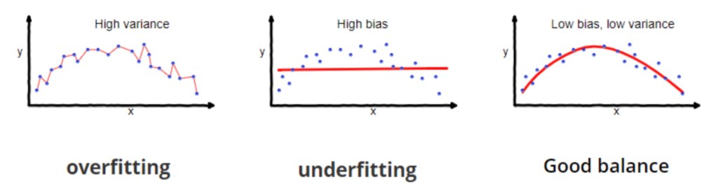
Part3: Bias & Variances TradeOFF

Consider that I answered a question wrong in an exam. There are two cases: the question is either in the mock or not. If the question is in the mock, the reason why I answered it wrong is that I didn’t pay enough attention to the mock. If the question is not in the mock, the reason why I answered it wrong is that I memorize every question in it and apply every detail of the answers to a completely different question in the exam.

Similarly, in prediction models, prediction errors can be decomposed into two main subcomponents: errors due to bias, and errors due to variance.
The machine either doesn’t study enough or study every detail from the training data. Either situation leads to a failure in the test data.

To be a lazy student or a overly-diligent student? That is the question. The answer is Balance.

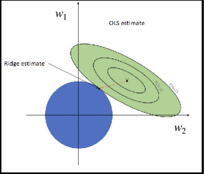
Part4: Ridge Regression

4.1 Invertibility of $XX^{T}$

In OLS, we get that $W = (XX^{T})^{-1}XY.$ But! What if $XX^{T}$ is not invertible? Could this happen? Hmmm. We need to recall from our Linear Algebra course. We know that $XX^{T}$ is a positive-semidefinite (PSD).

Proof: For any non-zero d*1 vector z:

$\displaystyle z^{T}(XX^{T})z = (X^{T}z)^{T}(X^{T}z) = ||(X^{T}z)||^{2} \geq 0$

But being PSD is not enough for being invertible. $XX^{T}$ need to be further positive-definite (PD) to be invertible.

Then for what X is $XX^{T}$ positive-definite? Or in other words, for what X does $XX^{T}$ evolve from PSD to PD?

Claim: X with full row rank makes $XX^{T}$ PD.

Proof:

Since X has full row rank, $X^{T}$ has full column rank. So $X^{T}$ has independent columns. The product $X^{T}z$ is a linear combination of the independent columns of $X^{T}$ . Then if $z \neq 0$ , $X^{T}z \neq 0$ . Thus for any non-zero d*1 vector z: $\displaystyle z^{T}(XX^{T})z = (X^{T}z)^{T}(X^{T}z) = ||(X^{T}z)||^{2} > 0$ .

Therefore, when d>n, X can’t be full row rank. Thus $XX^{T}$ is NOT invertible.

4.2 $XX^{T}$ and Motivation of Ridge Regression

When d>n, what could we do? $XX^{T}$ is only PSD. This is not enough. However, $\forall \lambda > 0, XX^{T} + \lambda I$ is PD.

Proof:

Suppose c is an eigenvalue of $XX^{T}$ . And c’s corresponding eigenvector is $v$ . Then we claim that $c+\lambda$ is also an eigenvalue of $XX^{T} + \lambda I$ . As $(XX^{T} + \lambda I)v = cv+\lambda v = (c + \lambda )v$ . Thus all the eigenvalues of $XX^{T} + \lambda I$ are in the form of $c_{i} + \lambda$ , which are positive. Thus $XX^{T} + \lambda I$ is PD.

Therefore, $XX^{T} + \lambda I$ is invertible. We define $W_{ridge} = (XX^{T} + \lambda I)^{-1}XY.$

The name ‘ridge’ refers to the shape along the diagonal of I.

4.3 Loss Function of Ridge Regression

We recover the loss function by starting from the solution $W_{ridge} = (XX^{T} + \lambda I)^{-1}XY$ .

$\displaystyle (XX^{T} + \lambda I) W_{ridge} = XY$ .

$\displaystyle 2(XX^{T} + \lambda I) W_{ridge} - 2XY = 0$ .

$\displaystyle \frac{\partial (W^{T}XX^{T}W - W^{T}XY - Y^{T}X^{T}W + Y^{T}Y)}{\partial W} + \frac{\partial \lambda ||W||^{2}}{\partial W}= 0$

$\displaystyle \frac{\partial || X^{T}W-Y ||^2}{\partial W} + \frac{\partial \lambda ||W||^{2}}{\partial W}= 0$

$\displaystyle || X^{T}W-Y ||^2 + \lambda ||W||^{2}$ = Loss function of Ridge Regression

= Loss function of OLS Regression + $\lambda ||W||^{2}$ .

Part5: Lasso Regression

5.1 Loss Function of Lasso Regression:

$\displaystyle || X^{T}W-Y ||^2 + \lambda ||W||$

5.2 Compared to Ridge Regression:

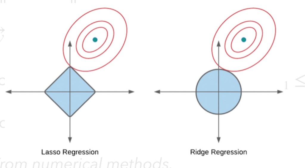
Because of diamond shape, the eclipse will often intersect it at each of the diamond corners. Due to that, at least one of the coefficients will equal zero. It serves as a method of eliminating features.

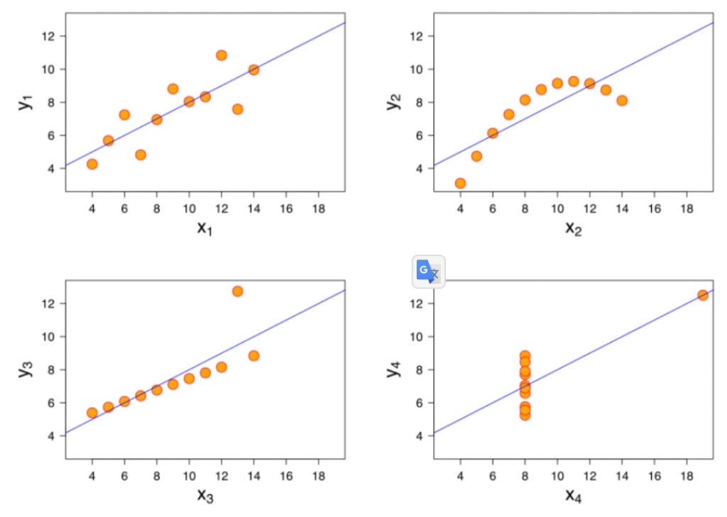
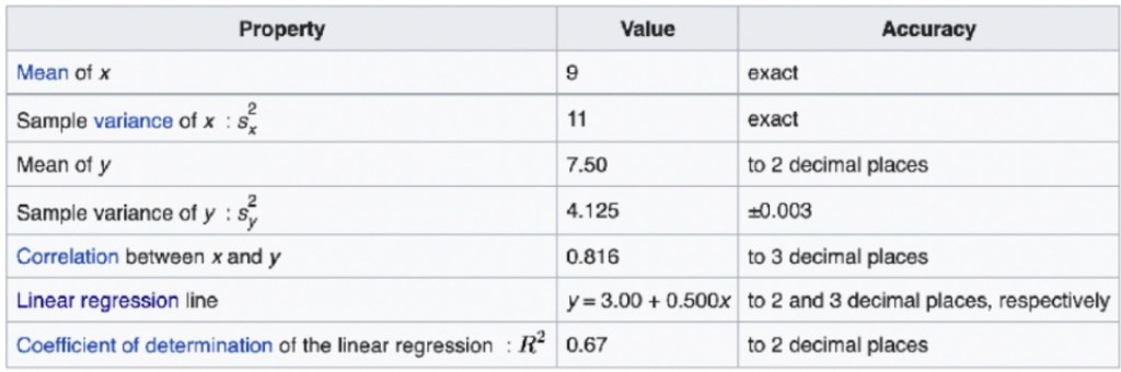
Part6: Numbers May Deceive You

A classic example of how numbers can deceive you if you don’t plot data out is Anscombe’s quartet.

2022年9月20日

Linear Regression

Regressions: From Linear to Ridge and Lasso